What survived our search for a cheaper neural-network estimator
A small spectral update, measured gains, and the limits that stayed in the result.
Adem Vessell · 22 October 2026 · Research case study
Knowing every weight in a neural network does not make its average response cheap to calculate. The Alignment Research Center (ARC) White-Box Estimation Challenge asks participants to estimate that response using the network’s structure, under a strict computation budget. Here, an estimator is a program that predicts the network’s average activations across random inputs. It is not a newly trained neural network.
I led an investigation into that problem with extensive AI assistance. Our submitted contribution became a small change to how an existing estimator compresses newly created interactions. It improved that estimator in matched local comparisons and completed official public grading. A stronger public competitor still performed substantially better.
The useful result is specific: using a standard matrix method to choose which interaction direction to retain improved this particular estimator, for very little added computation. That is the signed spectral update described below.
The problem: estimate an average without paying for every sample
The challenge uses known, randomly initialized networks with 16 layers, each containing 1,024 neurons. Each layer applies ReLU, which sets negative values to zero and leaves positive values unchanged. Inputs follow a Gaussian, or bell-shaped, distribution. The output to estimate is the mean activation of each neuron; the score uses final-layer error. Ordinary Monte Carlo repeatedly sends random inputs through the network and averages the answers. A white-box estimator can instead inspect the weights and propagate an approximation of the activation distribution. ARC’s research paper develops this approach.
The difficulty is deciding what survives each update. A mean and variance are compact, but later nonlinearities can depend on relationships those summaries omit. Keeping more relationships costs computation. Our estimator tracks selected higher-order interactions using cumulants: quantities that describe structure beyond a Gaussian approximation.
Raw mean squared error (MSE) averages the squared differences between the predicted means and the supplied reference estimates. For valid predictions, the challenge’s adjusted error multiplies final-layer MSE by a compute penalty: max(0.1, weighted prediction FLOPs / 2^41). FLOPs are floating-point arithmetic operations, weighted under the evaluator’s counting rules; they are not elapsed seconds. Lower adjusted error is better. Setup is the preparation before prediction, and has its own limits alongside memory and runtime. An accuracy gain must earn its full cost.
What we built, and what we inherited
We worked inside an estimator derived from ARC’s public cumulant-propagation method. It already tracked means, covariance—how pairs of activations vary together—and selected three-way and four-way interactions. It also already had machinery for carrying those summaries through layers and correcting selected quantities.
The parent estimator is our frozen comparison version of that program immediately before the spectral change, including its existing fourth-order approximations and computational optimizations. “Frozen” means the code was held unchanged for the comparison. This is a specific organizer-derived program, not ARC’s untouched reference implementation or the participant estimator V29.
Our change was a small part of that larger program: construct a richer description of newly created three-way interactions, compress it into one signed direction using standard spectral mathematics, and adapt the existing correction to match. The surrounding representation and layer-to-layer update machinery were retained. We did not build a replacement for the whole estimator.
The change: choose a better direction at birth
The inherited estimator stores cubic, or three-way, interaction information using groups of smaller numerical arrays called factors. At each layer except the final one, it creates a new group—a birth. Later layers transport these arrays through the network’s weights and query them to recover the particular interaction estimates needed for corrections.
For each center used to construct that group, two of the three factors can be summarized by the symmetric matrix below. This is a matrix used to build one cubic contribution, not the full array of three-neuron interactions:
M = h₀ uuᵀ + (uvᵀ + vuᵀ)/2
Here, u and v come from the estimator’s current covariance and higher-order approximations; h₀ comes from its ReLU update. The superscript ᵀ means transpose. Rank at most two means this matrix acts within at most two independent directions. We approximate it by one direction q with a signed weight λ, written λqqᵀ. Spectral refers to using the matrix’s eigenvectors—directions it maps to multiples of themselves. We choose the eigenvalue with largest absolute magnitude and its eigenvector; the retained weight can be positive or negative.

The matrix calculation reduces to a two-dimensional problem, using vector dot products and ordinary arithmetic. It avoids solving an eigenvalue problem across the full network width. The result fits the existing factor arrays—called panels in the diagram—so it adds no panel to carry forward and no matrix multiplication to the queries. Its extra work is quadratic in width: roughly four times as much when the width doubles. The complete estimator still pays to update all the history it retains.
We also adjust the inherited repair channel, an extra correction stored alongside the compressed information. It restores selected immediate third-order targets: D3 describes a single neuron’s asymmetric variation, while D21 describes the centered three-factor relationship in which one neuron appears twice and another once. In exact arithmetic, the repair matches the parent’s target formulas evaluated on the candidate’s current approximate state. Those targets are not the true network’s exact quantities, and later targets can differ from those of a separately evolved parent. Matching them does not guarantee later accuracy.
Choosing a dominant signed eigendirection is established mathematics. The local best-approximation result concerns this matrix considered on its own. It is not a theorem about the full three-way interaction array—a tensor—or final network error. That gap is why we needed comparison controls.
What the comparisons actually showed
The primary local comparison used three public networks, records 003–005, that had already been examined during our research. They were exposed cases, not unseen validation networks or holdouts. Every reported cost below covers the complete weighted prediction: history updates, interaction queries, conversions between numerical formats (casts), and the final output calculation (readout). Setup had separate acceptance limits; it is not silently counted as free.
V29 is a publicly shared neural-network estimator developed by challenge participant 504aldo. It propagates compact approximations of higher-order relationships through the network. We used it as a strong comparison method; it achieved lower adjusted error than our spectral candidate in the reported local study. 504aldo’s method explanation · Exact V29 source revision used in our comparison.
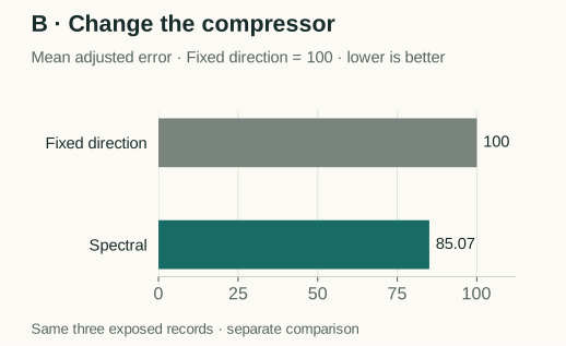
The charts answer two different questions:
- Parent comparison: does the complete change help? The parent used the
h₀uuᵀpart of the matrix above and omitted the terms involvingv. Our submitted version adds those terms and changes how the matrix is compressed. - Fixed-direction control: does choosing a new direction help once those extra terms are available? This comparison version uses the same source formulas as ours but keeps the original
udirection. It recalculates the best signed weight for that direction, rather than freezing the weight. Each version then evolves its own approximate state.
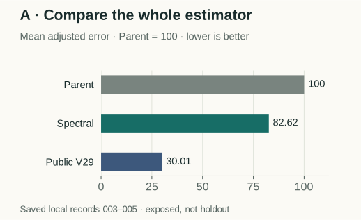
Against its parent: spectral’s mean adjusted error was 17.384% lower, for 0.05157% more prediction FLOPs. We averaged each method’s adjusted errors across the three primary networks, giving each network equal weight, then compared those averages. The full comparison ran three estimators on six exposed networks: 18 calls, all successful. The headline statistic uses the predeclared primary three-case subset.
Against a fixed-direction control: spectral reduced mean adjusted error by 14.929%, for 0.018790% more prediction FLOPs. This later comparison used the same three exposed networks, with six successful calls. Both arms used the same source-construction formulas and repair, but their evolving states could differ. It tests compressor choice within the recurrence, not identical saved inputs at every layer.
These percentages use different controls on overlapping cases. They cannot be added or compounded.
| Primary local comparison | Mean raw MSE ↓ | Mean adjusted error ↓ | Weighted prediction FLOPs ↓ |
|---|---|---|---|
| Frozen parent | 3.23746 × 10⁻⁸ | 1.97960 × 10⁻⁸ | 1.344633 trillion |
| Submitted spectral | 2.67328 × 10⁻⁸ | 1.63547 × 10⁻⁸ | 1.345327 trillion |
| Public V29 | 2.22462 × 10⁻⁸ | 5.94100 × 10⁻⁹ | 0.587263 trillion |
Our candidate was 2.753× worse than V29 on adjusted error in this comparison and about 2.291× as expensive. The result supports an improvement over our parent, with a separate control supporting the spectral selection. It does not establish a competitive lead.
The negative result that limits the claim
A transfer study asks whether a change helps when placed inside another estimator. We tested a restricted version of our spectral change inside V29 in a separate local study; that adapter was not submission #335293. Of four paired cases, one adapter call breached the evaluator’s separate 400 ms residual-time limit. The study also had a distinct 120-second limit for the whole prediction. All three valid pairs had worse raw MSE. Two had slightly better adjusted error because their cost was lower; that is not an accuracy improvement. We closed that route.
Small controls also exposed mathematical limits. Components can cancel each other; compressing each separately can disturb that cancellation. A locally best matrix approximation need not be best for the full three-way interaction array used later. Restoring the selected repeated-neuron quantities does not recover every interaction among three different neurons. Reference values were supplied dataset estimates, not proven exact expectations, and we did not newly quantify their uncertainty.
Those limits belong beside the positive result. The measured gain is real within the recorded comparison; generalization and stronger-estimator benefit remain unestablished.
What came from my earlier ideas—and what came from prior work
My earlier Crystal and provenance work kept returning to a question: what distinctions should an object retain so a later operation can still use them? Those ideas provided a conceptual lens and motivated a separate review of my earlier work. That review did not identify a usable ARC mechanism.
The submitted code does not run a Crystal algebra table, provenance decoder or learned compression language. Its representation is explicit numerical factors. The connection is a research question and design preference, not evidence that those earlier systems produced this gain.
The organizer’s cumulant method supplied the factorized cubic representation and the operations for transporting it, querying it and repairing selected repeated-neuron quantities (the identity-leg repair in the source code). Signed rank-one spectral approximation is standard. Protecting selected moments during low-rank approximation also has established precedents. Public participant 504aldo’s V18/V29 work informed our investigation and supplied the strong comparator. Our increment is the specified per-center source approximation and its matching repair subtraction. We make no first-use or exclusivity claim.
AI assistance was extensive. Under my research direction, Codex generated implementation, derivations, controls, analysis and most of the paper and this article. Other Codex agents challenged the work; the broader search also included Claude and Gemini. Claims were checked against code and recorded results. Agreement among AI agents is not independent human peer review.
What others can use
One practical output is Numerical Research Kit, a public plugin and open-source collection of deterministic comparison tools. It compares supplied baseline and candidate predictions against references, calculates error versus declared cost, bounds the possible benefit of a fixed correction, and helps freeze and verify study records.
It checks arithmetic and artifact integrity. The user still supplies the reference and cost evidence. It does not automatically measure compute, establish statistical confidence, or certify a scientific claim.
For researchers already working on factorized cumulant recurrences, the spectral update is a concrete approximation to inspect. For a broader engineering audience, the reusable lesson is the comparison itself: keep the strong baseline visible, separate accuracy from cost, preserve failures, and use a nearby control to find out what actually helped.
We finished with a graded estimator, a bounded contribution, and a reusable tool. Whether the approximation is valuable in other recurrences remains an open question. The existing results make that question precise enough to investigate.
Sources and attribution
- ARC: Wu et al., Estimating the expected output of wide random MLPs more efficiently than sampling, 2026; pinned organizer source.
- Spectral approximation: Zhang, Ling and Qi, The Best Rank-1 Approximation of a Symmetric Tensor and Related Spherical Optimization Problems, 2012; the order-two result is the relevant standard matrix case.
- Moment-preserving low-rank precedent: Guo and Qiu, A Conservative Low Rank Tensor Method for the Vlasov Dynamics.
- Participant comparator: 504aldo, Everything we tried: a factorized K=3 cumulant-propagation estimator; pinned V29 source.
- Reusable tooling: Numerical Research Kit, public plugin version 0.3.0.
This article summarizes the submitted spectral update and saved studies. No new numerical experiment was performed to prepare it. It is not a statement of organizer endorsement or an award.